
Knee Replacement
Introduction
In this section we will:
* identify which Knee Replacement procedures were excluded and why
* identify which different Knee Replacement subgroups were created and why
If you have questions or concerns about this data please contact Alexander Nielson (alexnielson@utah.gov)
Load Libraries
Load Libraries
library(data.table)
library(tidyverse)
## Warning: replacing previous import 'vctrs::data_frame' by 'tibble::data_frame'
## when loading 'dplyr'library(stringi)
library(ggridges)
library(broom)
library(disk.frame)
library(RecordLinkage)
library(googlesheets4)
library(bigrquery)
library(DBI)
devtools::install_github("utah-osa/hcctools2", upgrade="never" )
library(hcctools2)Establish color palettes
cust_color_pal1 <- c(
        "Anesthesia" = "#f3476f",
        "Facility" = "#e86a33",
        "Medicine Proc" = "#e0a426",
        "Pathology" = "#77bf45",
        "Radiology" = "#617ff7",
        "Surgery" = "#a974ee"
    )

cust_color_pal2 <- c(
        "TRUE" = "#617ff7",
        "FALSE" = "#e0a426"
    )

cust_color_pal3 <- c(
        "above avg" = "#f3476f",
        "avg" = "#77bf45",
        "below avg" = "#a974ee"
    )


  fac_ref_regex <- "(UTAH)|(IHC)|(HOSP)|(HOSPITAL)|(CLINIC)|(ANESTH)|(SCOPY)|(SURG)|(LLC)|(ASSOC)|(MEDIC)|(CENTER)|(ASSOCIATES)|(U OF U)|(HEALTH)|(OLOGY)|(OSCOPY)|(FAMILY)|(VAMC)|(SLC)|(SALT LAKE)|(CITY)|(PROVO)|(OGDEN)|(ENDO )|( VALLEY)|( REGIONAL)|( CTR)|(GRANITE)|( INSTITUTE)|(INSTACARE)|(WASATCH)|(COUNTY)|(PEDIATRIC)|(CORP)|(CENTRAL)|(URGENT)|(CARE)|(UNIV)|(ODYSSEY)|(MOUNTAINSTAR)|( ORTHOPEDIC)|(INSTITUT)|(PARTNERSHIP)|(PHYSICIAN)|(CASTLEVIEW)|(CONSULTING)|(MAGEMENT)|(PRACTICE)|(EMERGENCY)|(SPECIALISTS)|(DIVISION)|(GUT WHISPERER)|(INTERMOUNTAIN)|(OBGYN)"
Connect to GCP database
bigrquery::bq_auth(path = 'D:/gcp_keys/healthcare-compare-prod-95b3b7349c32.json')

# set my project ID and dataset name
project_id <- 'healthcare-compare-prod'
dataset_name <- 'healthcare_compare'

con <- dbConnect(
  bigrquery::bigquery(),
  project = project_id,
  dataset = dataset_name,
  billing = project_id
)
Get NPI table
query <-  paste0("SELECT npi, clean_name, osa_group, osa_class, osa_specialization
                 FROM `healthcare-compare-prod.healthcare_compare.npi_full`")

#bq_project_query(billing, query) # uncomment to determine billing price for above query.

npi_full <- dbGetQuery(con, query) %>%
  data.table()
get a subset of the NPI providers based upon taxonomy groups
gs4_auth(email="alexnielson@utah.gov")surgery <- read_sheet("https://docs.google.com/spreadsheets/d/1GY8lKwUJuPHtpUl4EOw9eriLUDG9KkNWrMbaSnA5hOU/edit#gid=0",
sheet="major_surgery") %>% as.data.table## Reading from "Doctor Types to Keep"## Range "'major_surgery'"surgery <- surgery[is.na(Remove) ] %>% .[["NUCC Classification"]] npi_prov_pair <- npi_full[osa_class %in% surgery] %>%
.[,.(npi=npi,
clean_name = clean_name
)
] Load Data
bun_proc <- disk.frame("full_apcd.df")knee <- bun_proc[surg_bun_t_knee == T & surg_bun_t_arthroplasty==T & surg_bun_sum_med > 2000]knee <- knee[duration_mean >=0]knee <- knee[,`:=`(
surg_sp_name_clean = surg_sp_npi %>% map_chr(get_npi_standard_name),
surg_bp_name_clean = surg_bp_npi %>% map_chr(get_npi_standard_name),
medi_sp_name_clean = medi_sp_npi %>% map_chr(get_npi_standard_name),
medi_bp_name_clean = medi_bp_npi %>% map_chr(get_npi_standard_name),
radi_sp_name_clean = radi_sp_npi %>% map_chr(get_npi_standard_name),
radi_bp_name_clean = radi_bp_npi %>% map_chr(get_npi_standard_name),
path_sp_name_clean = path_sp_npi %>% map_chr(get_npi_standard_name),
path_bp_name_clean = path_bp_npi %>% map_chr(get_npi_standard_name),
anes_sp_name_clean = anes_sp_npi %>% map_chr(get_npi_standard_name),
anes_bp_name_clean = anes_bp_npi %>% map_chr(get_npi_standard_name),
faci_sp_name_clean = faci_sp_npi %>% map_chr(get_npi_standard_name),
faci_bp_name_clean = faci_bp_npi %>% map_chr(get_npi_standard_name)
)]knee %>% saveRDS("knee.RDS")#stop hereknee <- readRDS("knee.RDS")We will first look at the distribution and high correlated tags.
knee %>% plot_med_density() %>% print()## `stat_bin()` using `bins = 30`. Pick better value with `binwidth`.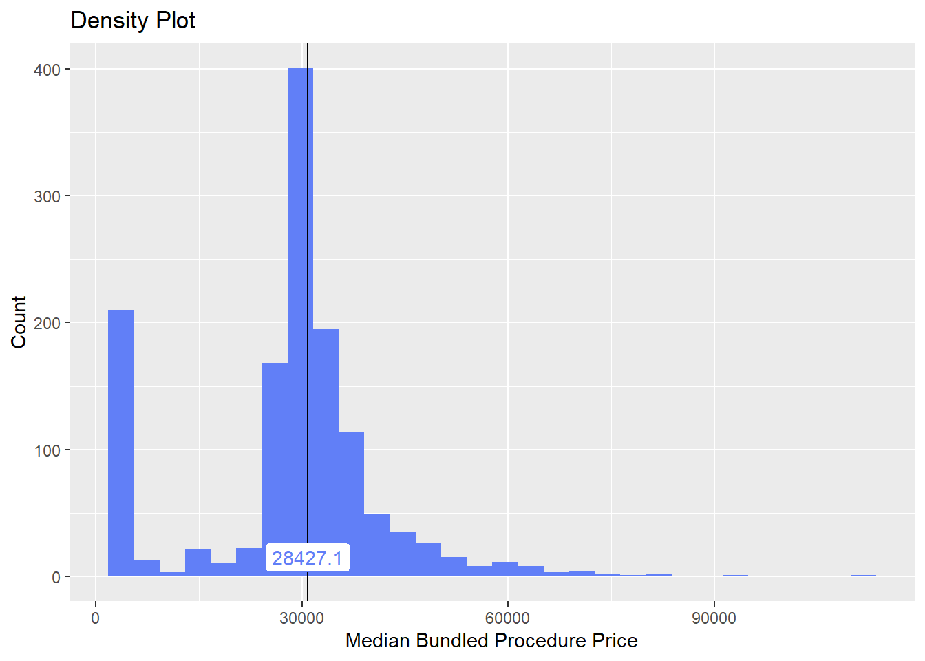
knee %>% get_tag_cor() %>% print()## Warning in stats::cor(cor_data): the standard deviation is zero## # A tibble: 210 x 2
## name correlation
## <chr> <dbl>
## 1 duration_mean 0.446
## 2 anes_bun_t_anes 0.260
## 3 anes_bun_t_anesth 0.260
## 4 anes_bun_t_knee 0.256
## 5 duration_max 0.160
## 6 path_bun_t_anti 0.138
## 7 path_bun_t_antibod 0.138
## 8 path_bun_t_typing 0.138
## 9 path_bun_t_screen 0.128
## 10 radi_bun_t_angiography 0.124
## # ... with 200 more rowsFirst thing to notice from the distribution is that we have a good chunk of knee surgeries that are under 5k. These are not reasonable estimates for the total knee replacements, and are likely only the surgeon costs (not the facility).
From the correlation table we can see that the duration is quite influential in the price as is reflected in higher facility costs.
Anesthesia presence also increases the cost.
Lets examine the duration vs median price visually:
knee %>% plot_price_vs_duration() %>% print()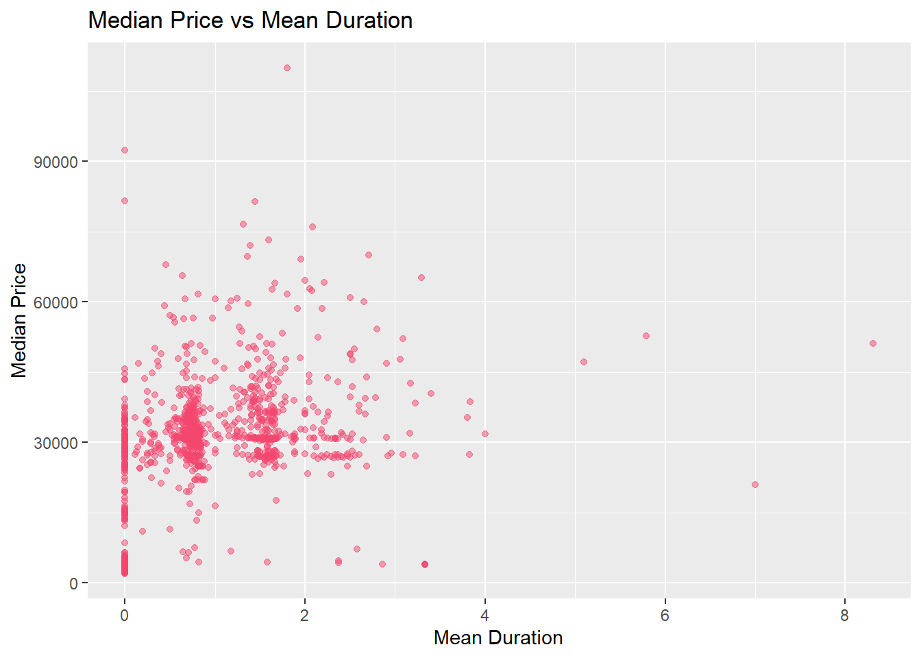
Lets see what happens if we remove any of the lower end prices, that are essentially missing facility costs. The below code will filter out any bundled procedures that have a facility cost under 1000.
knee <- knee[faci_bun_sum_med > 1000]knee %>% plot_med_density() %>% print()## `stat_bin()` using `bins = 30`. Pick better value with `binwidth`.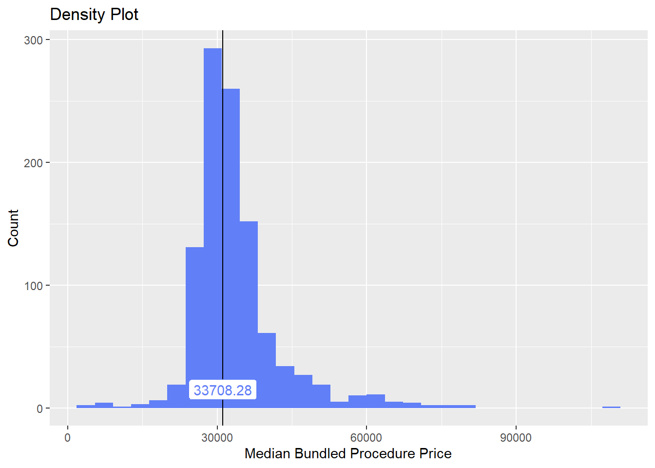
knee %>% get_tag_cor() %>% print()## Warning in stats::cor(cor_data): the standard deviation is zero## # A tibble: 190 x 2
## name correlation
## <chr> <dbl>
## 1 path_bun_t_anti 0.227
## 2 path_bun_t_antibod 0.227
## 3 path_bun_t_typing 0.227
## 4 path_bun_t_screen 0.199
## 5 duration_mean 0.199
## 6 radi_bun_t_angiography 0.191
## 7 path_bun_t_blood 0.169
## 8 path_bun_t_panel 0.166
## 9 path_bun_t_metabolic 0.159
## 10 faci_bun_t_hospital 0.150
## # ... with 180 more rowsthis looks much better. We still need to filter out non standard bundles, but this is a much mor expected distribution.
antibody typing
a pathology test that includes a antibody typing is higher correlated, so we will examine it
knee %>% get_tag_density_information("path_bun_t_antibod") %>% print()## Scale for 'y' is already present. Adding another scale for 'y', which will
## replace the existing scale.## Scale for 'x' is already present. Adding another scale for 'x', which will
## replace the existing scale.## [1] "tp_med ~ path_bun_t_antibod"## Warning in leveneTest.default(y = y, group = group, ...): group coerced to
## factor.## Picking joint bandwidth of 5580## $dist_plots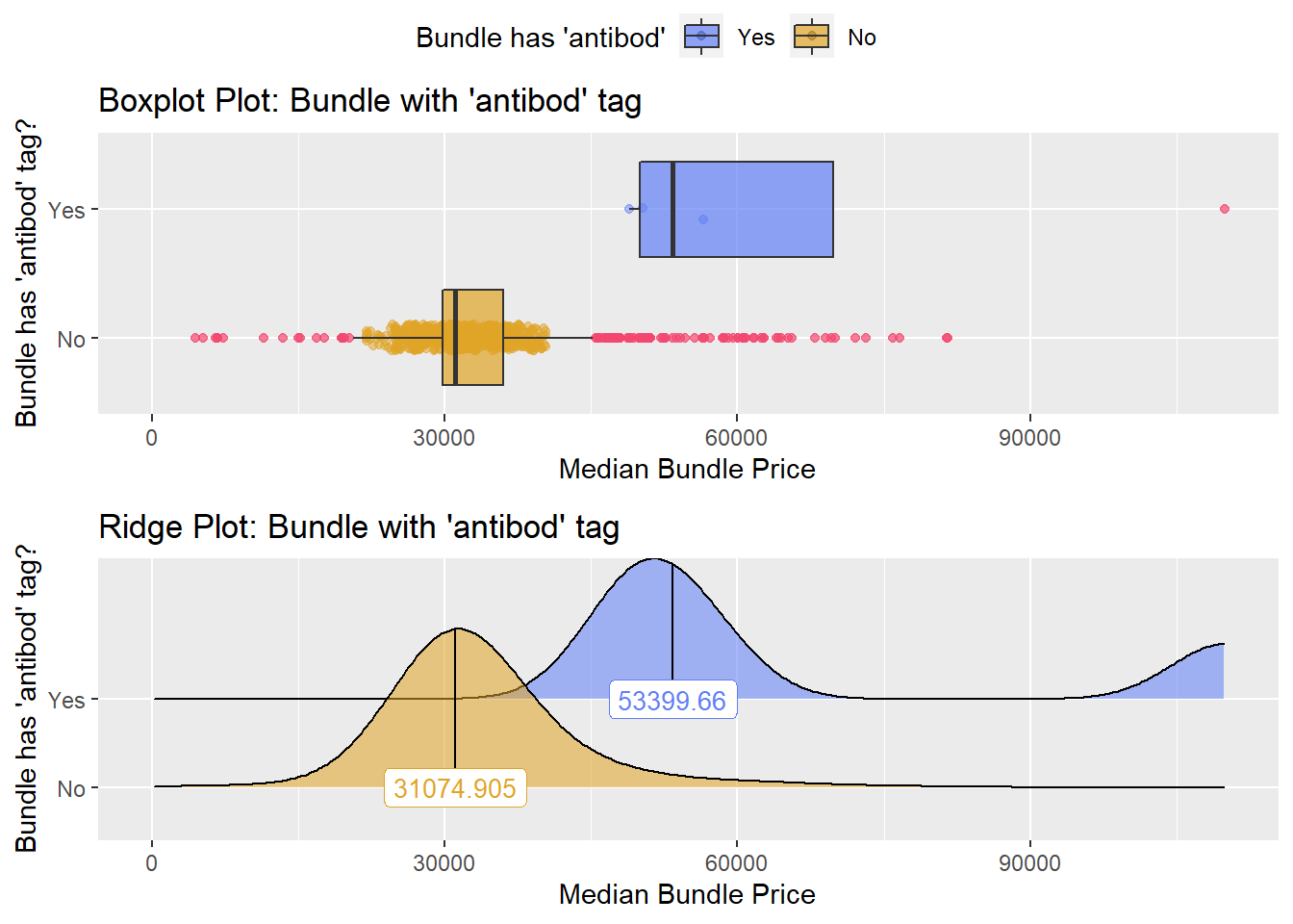
##
## $stat_tables
very few knee surgeries like this. It is not typical so they will be exluced from the standard
knee <- knee[path_bun_t_antibod==F]Once again lets look at the distribution of the knee surgeries with anesthesia and the correlated tags.
knee %>% plot_med_density() %>% print()## `stat_bin()` using `bins = 30`. Pick better value with `binwidth`.
knee %>% get_tag_cor() %>% print()## Warning in stats::cor(cor_data): the standard deviation is zero## # A tibble: 186 x 2
## name correlation
## <chr> <dbl>
## 1 duration_mean 0.202
## 2 surg_bun_t_femur 0.153
## 3 surg_bun_t_resect 0.153
## 4 surg_bun_t_tumor 0.153
## 5 faci_bun_t_hospital 0.134
## 6 faci_bun_t_care 0.128
## 7 faci_bun_t_subsequent 0.124
## 8 surg_bun_t_interlaminar 0.122
## 9 surg_bun_t_lamina 0.122
## 10 surg_bun_t_njx 0.122
## # ... with 176 more rowslets check the femur/resect/tumor bundle procs. I think this is rare so lets determine the number of surgeries like this:
knee[surg_bun_t_femur==T] %>% nrow()## [1] 1We can omit this one surgery from the standard.
knee <- knee [surg_bun_t_femur==F]Once again lets look at the distribution of the knee surgeries with anesthesia and the correlated tags.
knee%>% plot_med_density() %>% print()## `stat_bin()` using `bins = 30`. Pick better value with `binwidth`.
knee %>% get_tag_cor() %>% print()## Warning in stats::cor(cor_data): the standard deviation is zero## # A tibble: 183 x 2
## name correlation
## <chr> <dbl>
## 1 duration_mean 0.198
## 2 faci_bun_t_hospital 0.138
## 3 faci_bun_t_care 0.131
## 4 faci_bun_t_subsequent 0.127
## 5 radi_bun_t_echo 0.125
## 6 surg_bun_t_interlaminar 0.124
## 7 surg_bun_t_lamina 0.124
## 8 surg_bun_t_njx 0.124
## 9 radi_bun_t_guide 0.124
## 10 anes_bun_t_knee 0.121
## # ... with 173 more rowsfacility charge with “subsequent hospital care”
knee %>% get_tag_density_information("faci_bun_t_subsequent") %>% print()## Scale for 'y' is already present. Adding another scale for 'y', which will
## replace the existing scale.## Scale for 'x' is already present. Adding another scale for 'x', which will
## replace the existing scale.## [1] "tp_med ~ faci_bun_t_subsequent"## Warning in leveneTest.default(y = y, group = group, ...): group coerced to
## factor.## Picking joint bandwidth of 1300## $dist_plots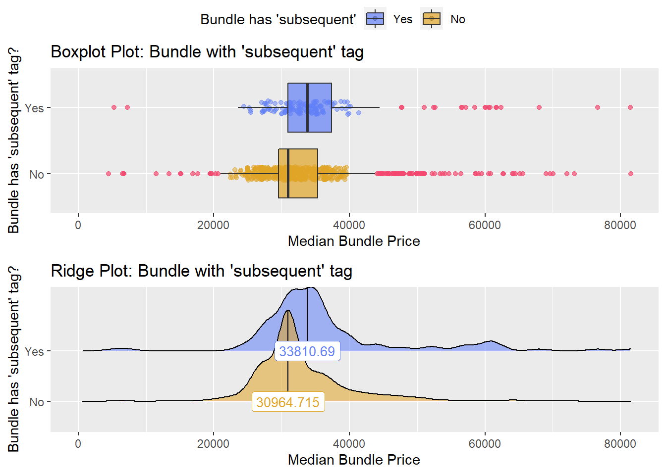
##
## $stat_tables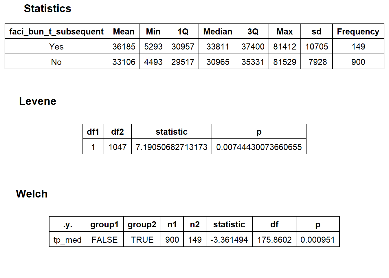
knee_at_sub_hosp <-  knee [faci_bun_t_subsequent==T]
knee <- knee[faci_bun_t_subsequent==F]
Once again lets look at the distribution of the knee surgeries with anesthesia and the correlated tags.
knee%>% plot_med_density() %>% print()## `stat_bin()` using `bins = 30`. Pick better value with `binwidth`.
knee %>% get_tag_cor() %>% print()## Warning in stats::cor(cor_data): the standard deviation is zero## # A tibble: 148 x 2
## name correlation
## <chr> <dbl>
## 1 duration_mean 0.194
## 2 surg_bun_t_interlaminar 0.126
## 3 surg_bun_t_lamina 0.126
## 4 surg_bun_t_njx 0.126
## 5 anes_bun_t_anes 0.111
## 6 anes_bun_t_anesth 0.111
## 7 surg_bun_t_dev 0.111
## 8 surg_bun_t_device 0.111
## 9 surg_bun_t_drug 0.111
## 10 surg_bun_t_remove 0.111
## # ... with 138 more rowsInterlaminar Injection
knee %>% get_tag_density_information("surg_bun_t_lamina") %>% print()## Scale for 'y' is already present. Adding another scale for 'y', which will
## replace the existing scale.## Scale for 'x' is already present. Adding another scale for 'x', which will
## replace the existing scale.## [1] "tp_med ~ surg_bun_t_lamina"## Warning in leveneTest.default(y = y, group = group, ...): group coerced to
## factor.## Picking joint bandwidth of 1960## $dist_plots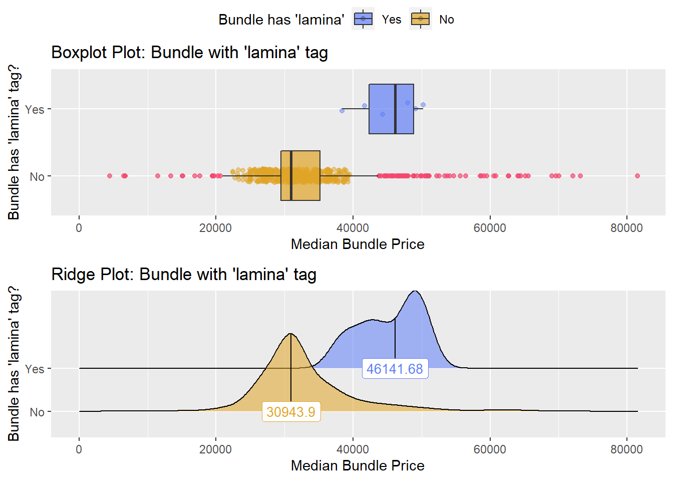
##
## $stat_tables
there is not enough observations to warrant a separate group, but there is a signficnat difference in the types, so they will be excluded from the standard pool.
knee <- knee[surg_bun_t_lamina==F]Once again lets look at the distribution of the knee surgeries with anesthesia and the correlated tags.
knee%>% plot_med_density() %>% print()## `stat_bin()` using `bins = 30`. Pick better value with `binwidth`.
knee %>% get_tag_cor() %>% print()## Warning in stats::cor(cor_data): the standard deviation is zero## # A tibble: 145 x 2
## name correlation
## <chr> <dbl>
## 1 duration_mean 0.190
## 2 surg_bun_t_dev 0.113
## 3 surg_bun_t_device 0.113
## 4 surg_bun_t_drug 0.113
## 5 surg_bun_t_remove 0.113
## 6 path_bun_t_without_scope 0.112
## 7 anes_bun_t_anes 0.110
## 8 anes_bun_t_anesth 0.110
## 9 anes_bun_t_knee 0.107
## 10 radi_bun_t_echo 0.104
## # ... with 135 more rowsknee[surg_bun_t_device==T] %>% nrow()## [1] 1the number of bundled procedures that have a device removal is too rare.
knee <- knee[surg_bun_t_device==F]Once again lets look at the distribution of the knee surgeries with anesthesia and the correlated tags.
knee%>% plot_med_density() %>% print()## `stat_bin()` using `bins = 30`. Pick better value with `binwidth`.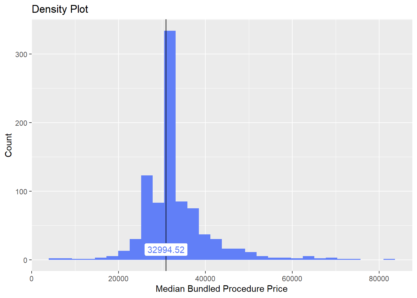
knee %>% get_tag_cor() %>% print()## Warning in stats::cor(cor_data): the standard deviation is zero## # A tibble: 141 x 2
## name correlation
## <chr> <dbl>
## 1 duration_mean 0.190
## 2 path_bun_t_without_scope 0.112
## 3 anes_bun_t_anes 0.110
## 4 anes_bun_t_anesth 0.110
## 5 anes_bun_t_knee 0.107
## 6 surg_bun_t_place 0.103
## 7 surg_bun_t_revise 0.103
## 8 radi_bun_t_echo 0.101
## 9 radi_bun_t_guide 0.101
## 10 medi_bun_t_sodium 0.0951
## # ... with 131 more rowsknee[path_bun_t_without_scope==T] %>% nrow()## [1] 1knee[surg_bun_t_revise==T] %>% nrow()## [1] 2knee <- knee[path_bun_t_without_scope==F & surg_bun_t_revise==F]Once again lets look at the distribution of the knee surgeries with anesthesia and the correlated tags.
knee%>% plot_med_density() %>% print()## `stat_bin()` using `bins = 30`. Pick better value with `binwidth`.
knee %>% get_tag_cor() %>% print()## Warning in stats::cor(cor_data): the standard deviation is zero## # A tibble: 138 x 2
## name correlation
## <chr> <dbl>
## 1 duration_mean 0.191
## 2 radi_bun_t_echo 0.113
## 3 radi_bun_t_guide 0.113
## 4 anes_bun_t_anes 0.112
## 5 anes_bun_t_anesth 0.112
## 6 anes_bun_t_knee 0.109
## 7 path_bun_t_panel 0.100
## 8 surg_bun_t_block 0.0997
## 9 medi_bun_t_sodium 0.097
## 10 medi_bun_t_sulfate 0.0958
## # ... with 128 more rowsknee %>% get_tag_density_information("radi_bun_t_echo") %>% print()## Scale for 'y' is already present. Adding another scale for 'y', which will
## replace the existing scale.## Scale for 'x' is already present. Adding another scale for 'x', which will
## replace the existing scale.## [1] "tp_med ~ radi_bun_t_echo"## Warning in leveneTest.default(y = y, group = group, ...): group coerced to
## factor.## Picking joint bandwidth of 1080## $dist_plots
##
## $stat_tables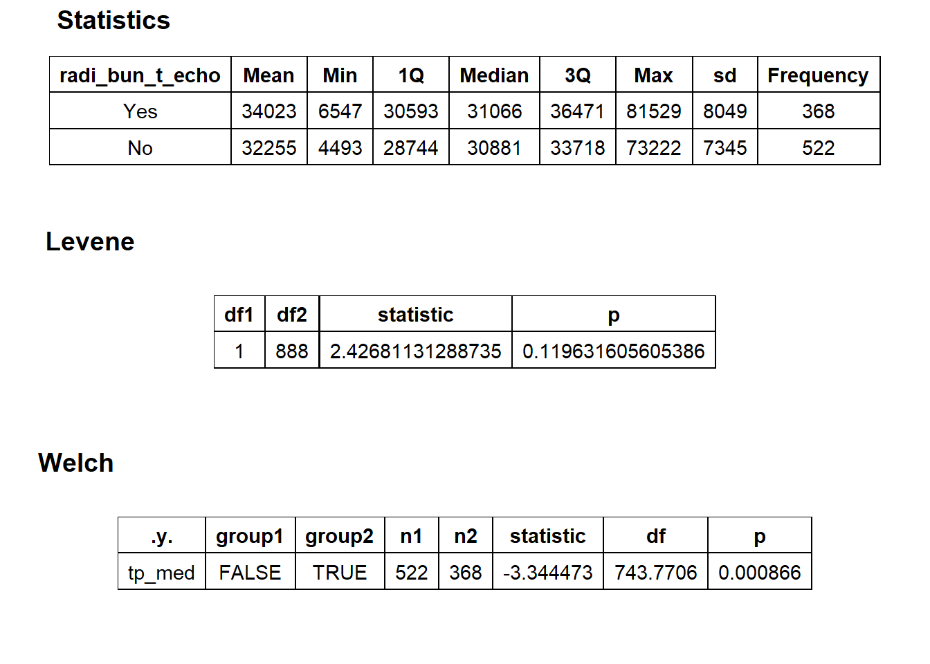
knee%>% plot_med_density() %>% print()## `stat_bin()` using `bins = 30`. Pick better value with `binwidth`.
knee %>% get_tag_cor() %>% print()## Warning in stats::cor(cor_data): the standard deviation is zero## # A tibble: 138 x 2
## name correlation
## <chr> <dbl>
## 1 duration_mean 0.191
## 2 radi_bun_t_echo 0.113
## 3 radi_bun_t_guide 0.113
## 4 anes_bun_t_anes 0.112
## 5 anes_bun_t_anesth 0.112
## 6 anes_bun_t_knee 0.109
## 7 path_bun_t_panel 0.100
## 8 surg_bun_t_block 0.0997
## 9 medi_bun_t_sodium 0.097
## 10 medi_bun_t_sulfate 0.0958
## # ... with 128 more rowsknee_btbv4 <- knee %>% btbv4()Get primary doctors
knee_final_bq <- knee_btbv4[,
                     primary_doctor := pmap(.l=list(doctor_npi1=doctor_npi_str1,
                                  doctor_npi2=doctor_npi_str2,
                                  class_reqs="Orthopaedic Surgery"
                                  ),
                                                .f=calculate_primary_doctor) %>% as.character()
                     ] %>%
  #Filter out any procedures where our doctors fail both criteria.
  .[!(primary_doctor %in% c("BOTH_DOC_FAIL_CRIT", "TWO_FIT_ALL_SPECS"))] %>%
  .[,primary_doctor_npi := fifelse(primary_doctor==doctor_str1,
                                   doctor_npi_str1,
                                   doctor_npi_str2)] %>%
  .[,`:=`(
    procedure_type=2,
    procedure_modifier = "Standard Knee Replacement"
  )]
## [1] "multiple meet class req"
## [1] "JEREMY MARK GILILLAND" "STEVEN DONOHOE"
## [1] "multiple meet class req"
## [1] "CHRISTOPHER EARL PELT" "STEVEN DONOHOE"
## [1] "multiple meet class req"
## [1] "CHRISTOPHER L. PETERS" "MICHAEL CHAD MAHAN"
## [1] "multiple meet class req"
## [1] "BRYAN C KING" "DAVID P MURRAY"
## [1] "multiple meet class req"
## [1] "BRANDON J FERNEY" "MICHAEL HAWKES METCALF"
## [1] "multiple meet class req"
## [1] "CHRISTOPHER L. PETERS" "KEVIN CAMPBELL"
## [1] "multiple meet class req"
## [1] "CHRISTOPHER L. PETERS" "STEVEN DONOHOE"
## [1] "multiple meet class req"
## [1] "THOMAS O HIGGINBOTHAM" "DAVID P MURRAY"
## [1] "multiple meet class req"
## [1] "CHRISTOPHER EARL PELT" "MICHAEL CHAD MAHAN"
## [1] "multiple meet class req"
## [1] "PETER SILVERO" "ROSS M JARRETT"
## [1] "multiple meet class req"
## [1] "JOSHUA M HICKMAN" "CLINT JOHN WOOTEN"
## [1] "multiple meet class req"
## [1] "JEREMY MARK GILILLAND" "KEVIN CAMPBELL"knee_final_bq <- knee_final_bq[,.(
primary_doctor,
primary_doctor_npi,
most_important_fac ,
most_important_fac_npi,
procedure_type,
procedure_modifier,
tp_med_med,
tp_med_surg,
tp_med_medi,
tp_med_path,
tp_med_radi,
tp_med_anes,
tp_med_faci,
ingest_date = Sys.Date()
)]bq_table_upload(x=procedure_table, values= knee_final_bq, create_disposition='CREATE_IF_NEEDED', write_disposition='WRITE_APPEND')